Modeling the dynamics of multi-species systems with the generalized Lotka-Volterra model
Aim of the work
The dynamics of multiple interacting species is often complex and the consequences of perturbation of large ecosystems are difficult to predict. Mathematical modeling gives insights on the structure-stability-dynamics relationships and help to interpret experimental observations.
The aim of this work is to simulate the generalized Lotka-Volterra (gLV) model and to analyze some dynamical properties of multi-species systems.
The multi-species Lotka-Volterra model
The generalized Lotka-Volterra (gLV) model simulates the time evolution of a multi-species system:
What do the parameters bi and aij represent?
Answer: bi are the intrinsic growth rates, and aij are the pairwise interaction coefficients. Parameters aii account for the intra-species interaction.
The above equation can be rewritten in matricial form:
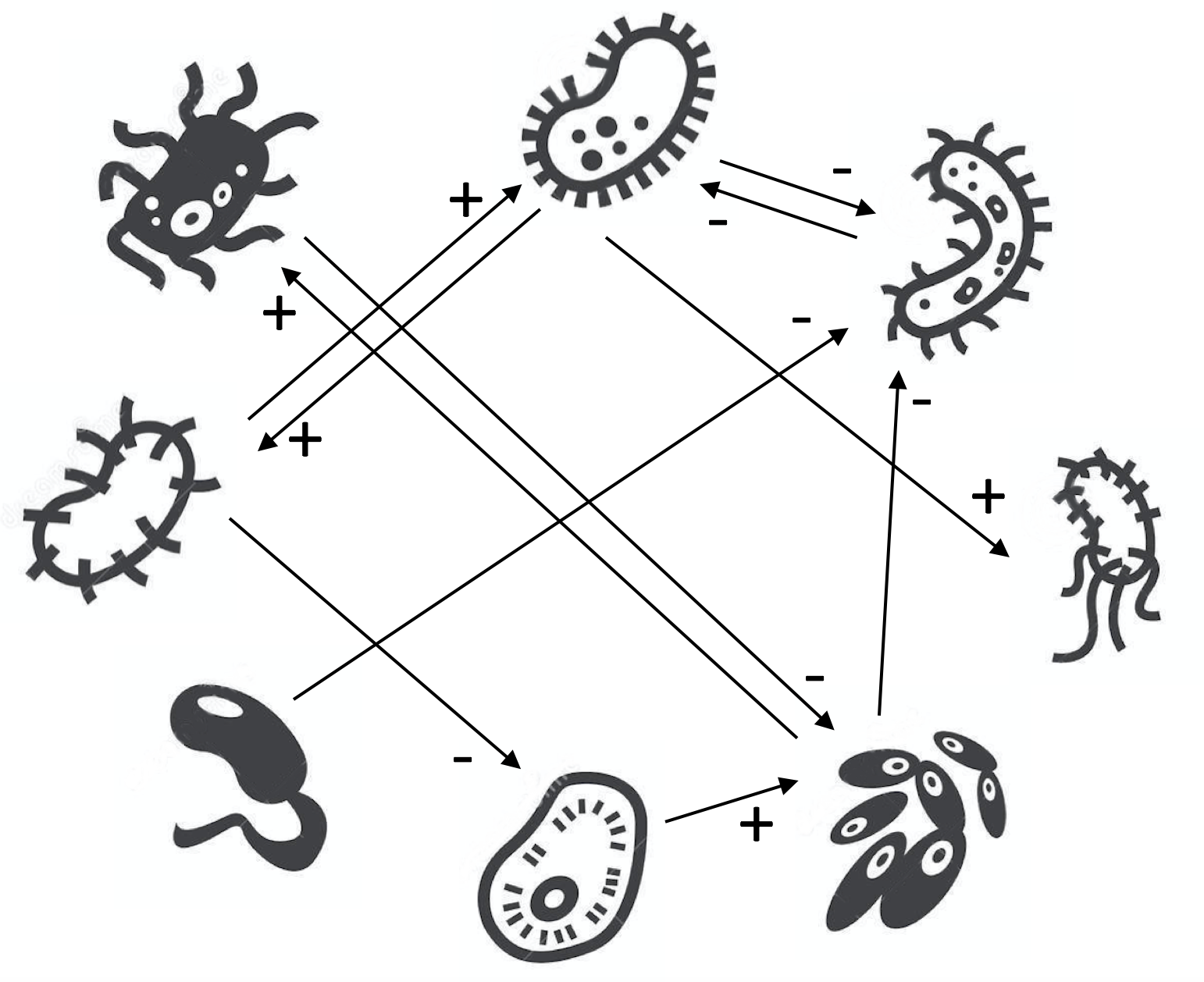
Write matrix A for the following microbial network:
Answer:
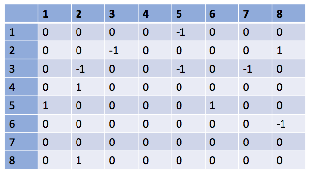
Remarks:
There are different types of interactions: mutualism (species 2-8), competition (2-3), parasitism, etc.
Species 4 in only an output - it does not influence the dynamics of the other species.
Note that self-interactions are not indicated in this matrix (the diagonal terms are set to 0). In practice, to account for intra-species competition and to avoid unlimited growth, the terms on the diagonal take negative value.
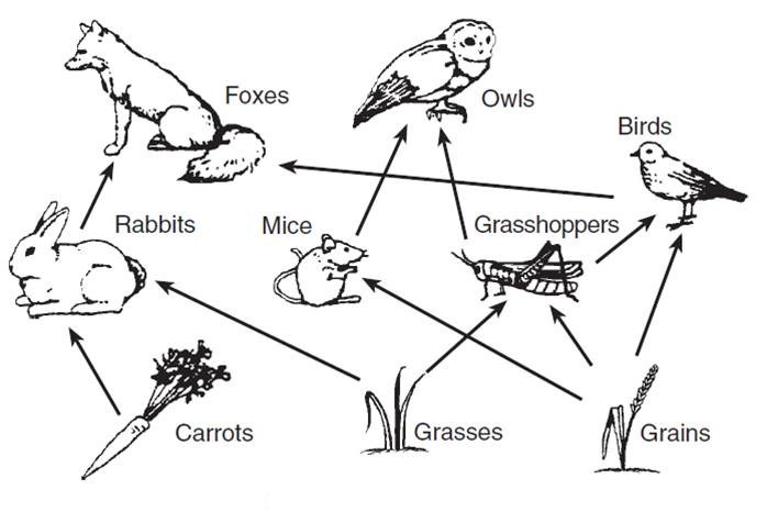
How does the matrix A look like for trophic food web (such as the one depicted on this figure)?
Answer: For trophic food webs, assuming that there no competition, the matrix is symetric and contains positive (or null) terms on the upper triangle and negative terms on the bottom triangle.

How could we theoretically calculate the steady state of the system? What it the potential problem with this calculation?
Answer: Theoretically the steady state, defined by dN/dt=0 can be calculated as Ns=-A-1b. This gives the non-trivial solution. The problem is that some values can be negative, which is unrealistic. This is due to the fact that some species may be dead (=0) at steady state. Thus the actual stable steady state is not the non-trivial one.
Simulation of the gLV model
Run simulations of the gLV model and discuss the effect of model parameters (number of species N, type and connectance of the interaction matrix, initial abundance, etc).
Answer:
| R code (librairies) |
library(devtools)

library(seqtime)
|
| R code |
N=50 # size of the population
A=generateA(N=N) # generate interaction matrix
R=glv(N=N,A=A) # run simulation
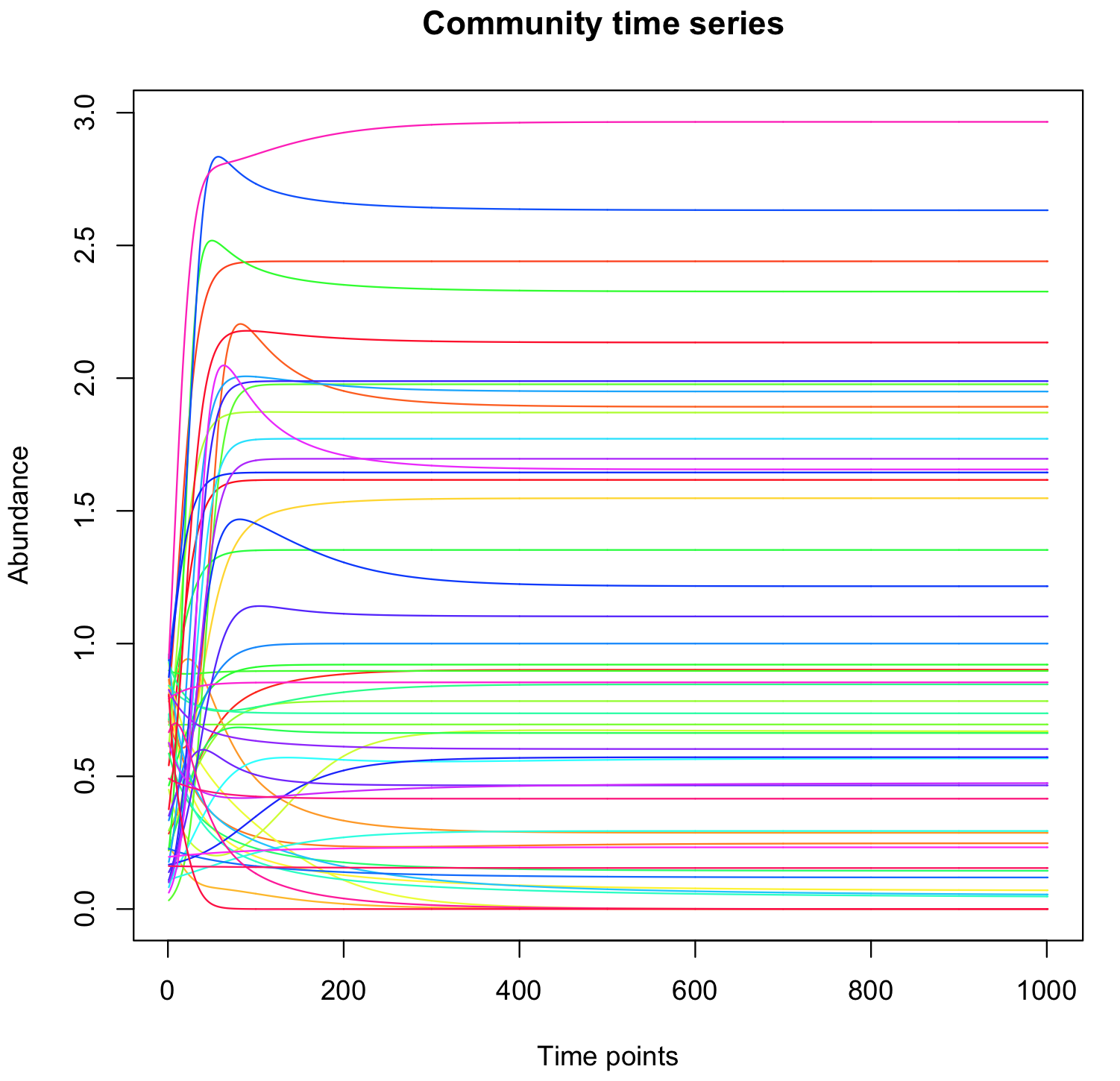
tsplot(R) # plot time series
|
You can then change the parameters to generate various interaction matrices A.
| R code |
N=50                                            # size of the population

A=generateA(N,d=-2,c=0.5,pep=20)  # generate a matrix with value "-1" on the diagonal
                                    # connectance:0.5, percent of positive edges=20

b=runif(N)                        # intrinsic growth rartes

yini=runif(N)                     # initial abundances

R=glv(N=N,A=A,b=b,y=yini)         # run simulation

tsplot(R) 		                        # plot time series
|
Some observations:
There is a relatively large proportion of species that spontaneously get extinct.
Changing the initial abundances does not change the steady state abundances, unless some species are initially set arbitrarily to zero.
Increasing the connectance decreases the survival rate.
With random network, when the proportion of positive interactions (ppe) is low, the steady states are lower and more species die. When the ppe is too high, we get "explosion" (some species grow indefinitely). this can be compensated by increasing the value of the terms on the diagonal. In that case, all species survive.
Species number vs survival rate
As you may have seen in your previous simulations, some species tends to die. Are bigger populations (i.e. population involving more species) more susceptible to species loss? To test this, you can compute and plot the survival rate as a function of the number of species. How do the type and connectance of the interaction matrix affect the observed tendancy. How does the positive vs negative interaction ratio influence the results?
Answer:
| R code |
Nmin=20

Nmax=200

Nint=20


NN=seq(Nmin,Nmax,by=Nint);         # range of N

SR=c();                            # initialize 'results' vector


for(N in NN){


print(paste(cat("\n"),"Run analysis for N =",N))


A=generateA(N=N);


R=glv(N=N,A=A)


th=0.01                            # threshold to determine if a species is alive or not.

s=length(which(R[,ncol(R)]>th))/N    # compute survial rate


print(paste("Survival rate =",s))


SR <- c(SR, s);


}    # end loop on N


plot(NN,SR,ylim = 0:1,xlab = "Number of species, N", ylab = "Survival rate", type = "l")
|
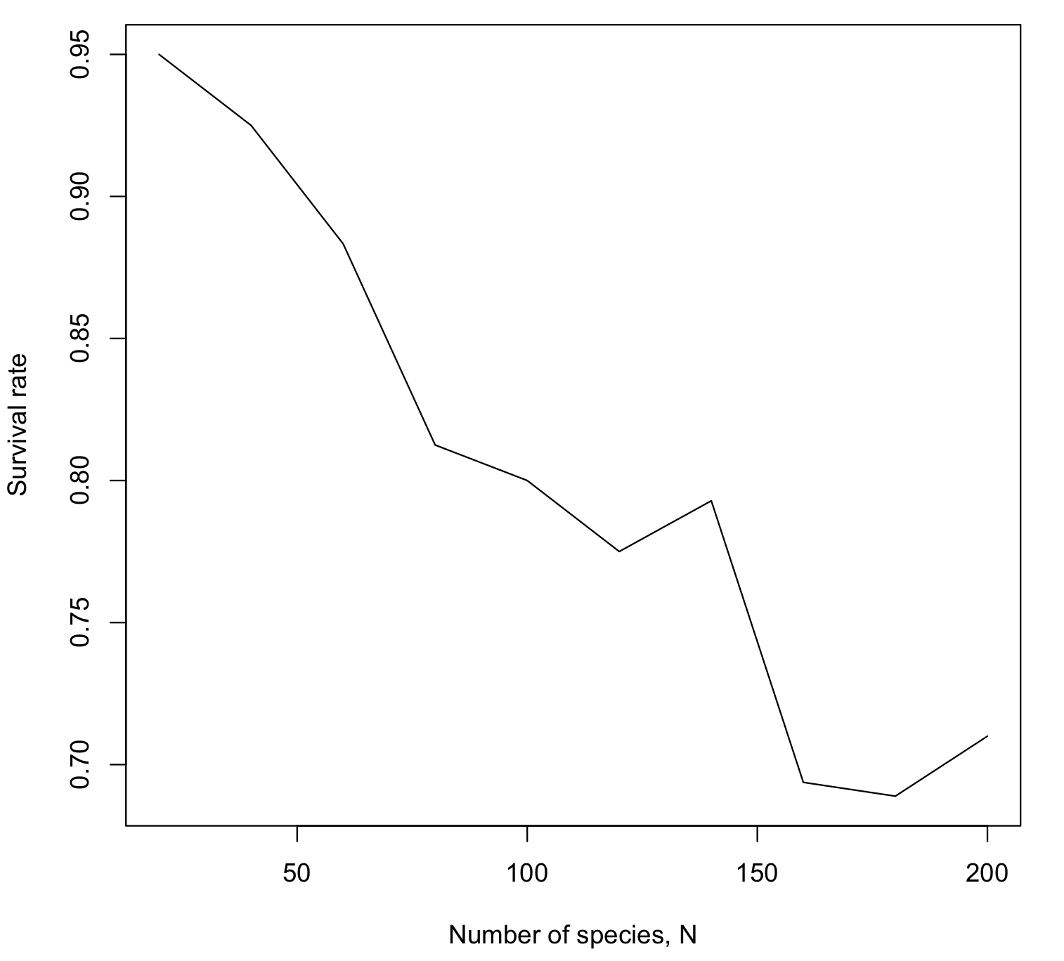
Some observations:
Increasing the number of species decreases the survival rate (as seen on the figure).
Increasing the connectance decreases the survival rate (run simulation for various values of c).
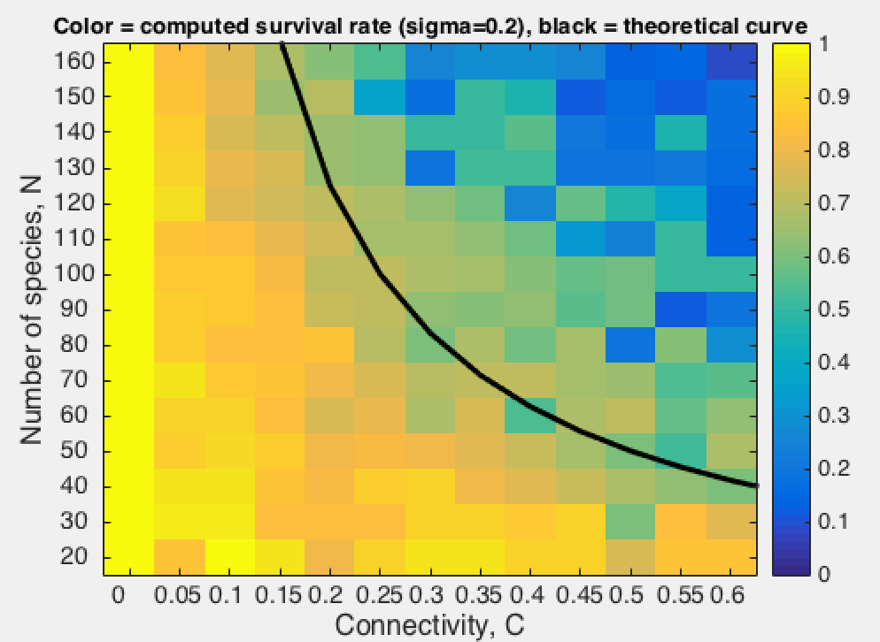
Wigner-May theorem
The above results suggest that stability is associated with complexity. Much work has been done to characterize these relationships and to identify the ecological factors that affect population stability. One key theoretical results, reported by May (1972) and known as the Wigner-May relationship, is the following: Using the gLV equations, May analyzed the probability P(S,α,C) for a system composed of S species with connectivity C (with 0 < C < 1) to be stable. For an interaction matrix A where the elements are drawn from a Normal distribution with mean 0 and standard deviation α, May established that:
Rather that to check the above relationship, we propose here to compute the survival rate as a function of S and C for various values of α.
Answer:
| R code |
Nmin=20;Nmax=160;Nint=20

Cmin=0;Cmax=0.6;Cint=0.1


NN=seq(Nmin,Nmax,by=Nint);     # range of N

CC=seq(Cmin,Cmax,by=Cint);     # range of C


SR <- matrix(data=NA,nrow=length(NN),ncol=length(CC))


i=0

for(N in NN){

i=i+1

j=0

for(c in CC){

j=j+1


print(paste(cat("\n"),"Run analysis for N = ",N," and c = ",c))


A=generateA(N=N,c=c);


R=glv(N=N,A=A)


th=0.001                            # threshold to determine if a species is alive or not.

s=length(which(R[,ncol(R)]>th))/N    # compute survial rate


print(paste("Survival rate =",s))


SR[i,j] = s;


}    # end loop on c

}    # end loop on N


image(SR,xlab = "Number of species, N", ylab = "Connectance, C", axes=FALSE)

axis(1,at=seq(from=0, to=1, by=1/(length(NN)-1)),labels=NN,srt=45,tick=FALSE)

axis(2,at=seq(from=0, to=1, by=1/(length(CC)-1)),labels=CC,srt=45,tick=FALSE)
|
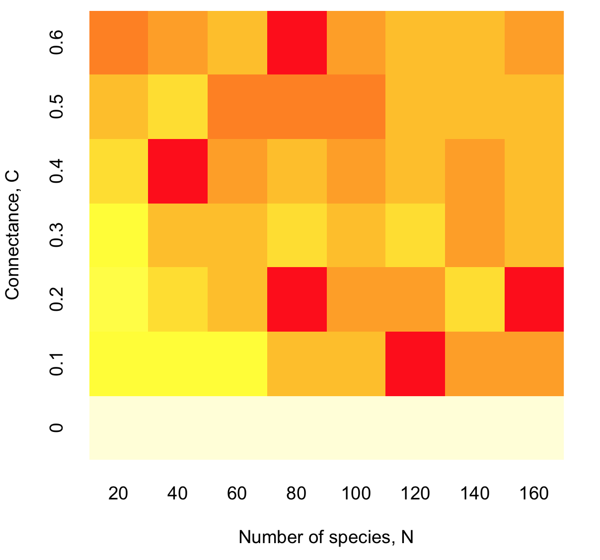
Some observations:
The survival rate seems to follow the tendancy predicted by Wigner and May (although more simulations and statistic are needed to support this observation - see here the results of a more detailed computation).
Interestingly, this tendancy is here observed for the case of "random" interaction matrices whereas Wigner and May derived the criteria for a matrix with normally distributed values.
Remark:
These observations raise a central question in ecology: Which factors may "stabilize" large ecological networks (thus allowing multiple species to live together).
Chaos
Chaos can be generated by coupling oscillatory systems. Show that chaos can be obtained in a mutually coupled predator-prey systems:
This can be done in 2 steps:
(1) Parametrize a 4-species system so that it correspond to 2 independent predator-prey systems.
(2) Introduce a (small) coupling between the 2 systems.
Chaos is characterized by its sensitivity to initial conditions. Run simulation from two close initial conditions and observe the divergence (decorrelation) of the trajectories (butterfly effect).
Answer:
Parameters for 2 independent predator-prey systems
b=[1 -1 1 -1];
A=[
| 0 | -1 | 0 | 0 |
| 1 | 0 | 0 | 0 |
| 0 | 0 | 0 | -1 |
| 0 | 0 | 1 | 0 |
]
A weak coupling could be introduced as follows:
A=[
| 0 | -1 | 0 | 0 |
| 1 | 0 | -0.2 | 0 |
| 0 | 0 | 0 | -1 |
| 0 | 0.2 | 1 | 0 |
]
| R code |
b=c(1,-1,1,-1)
A=array(c(0,-1,0,0,1,0,0,-0.2,0,0,0,-1,0,0.2,1,0),c(4,4))
A=t(A)
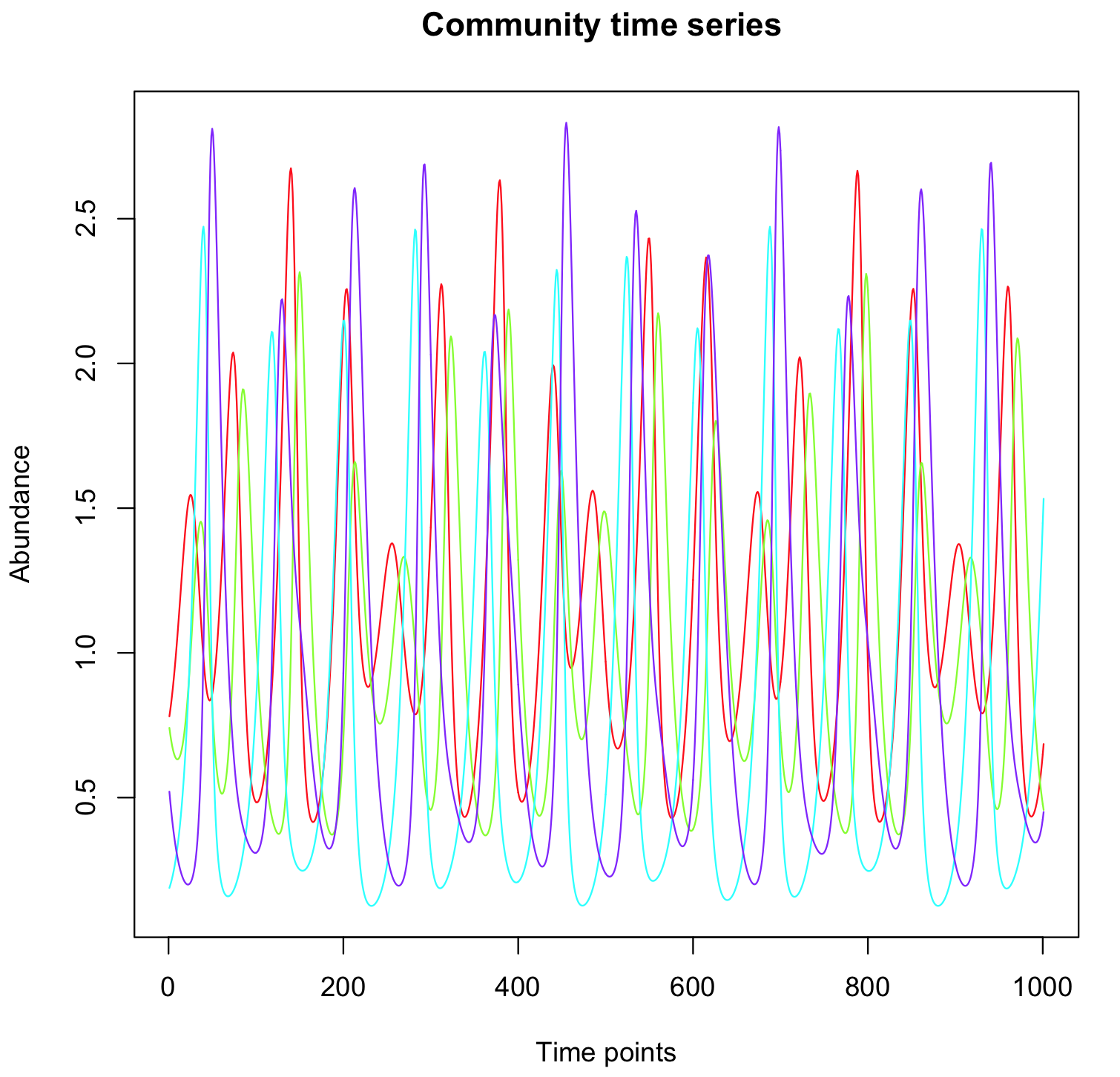
R=glv(N=4,A=A,b=b,tend=100)
tsplot(R)
|
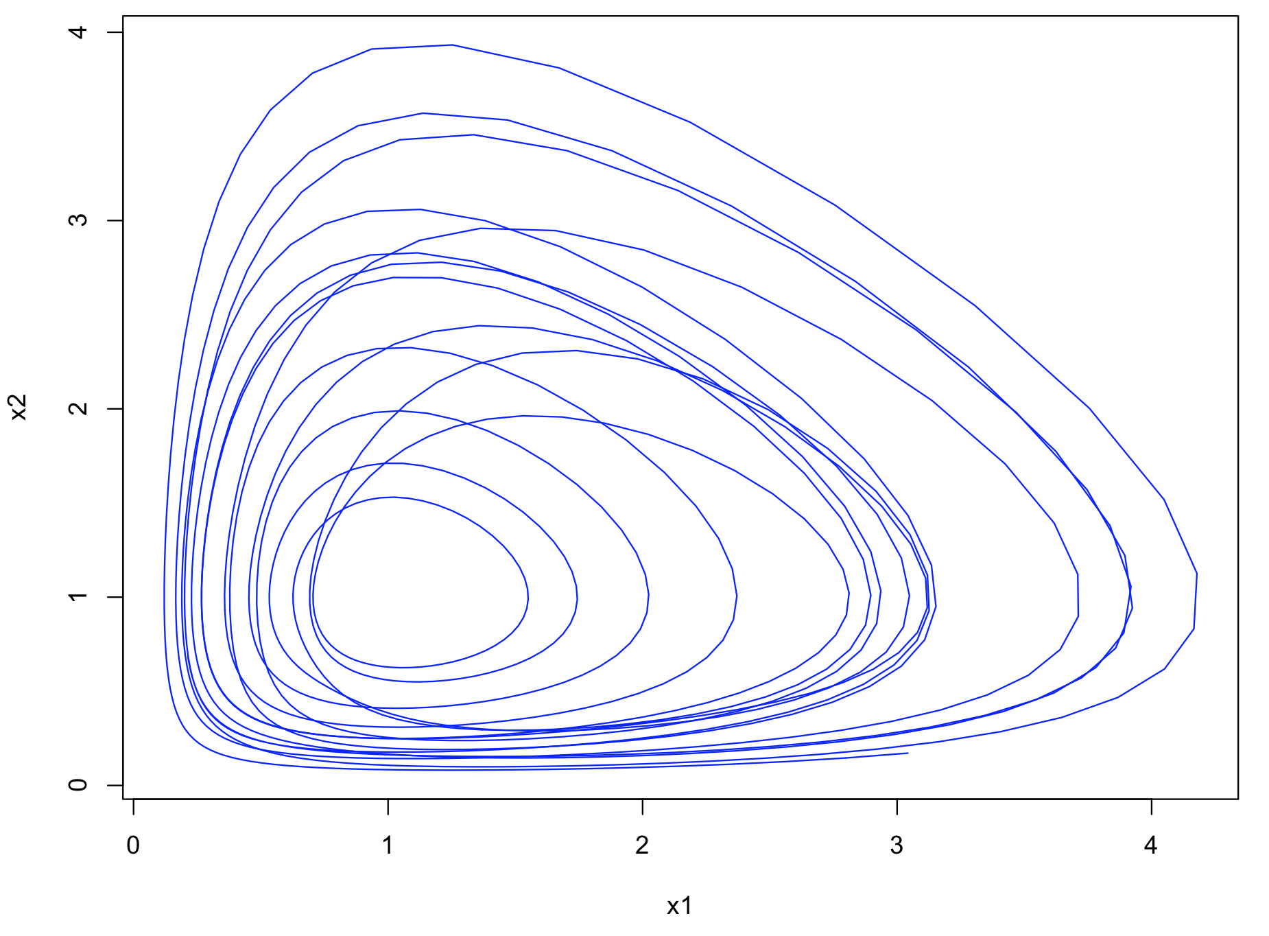
The trajectory in the phase space (= attractor) can be plot as follows:
| R code |
plot(as.numeric(R[1,]),as.numeric(R[2,]), col="blue", type="l", xlab="x1", ylab="x2")
|
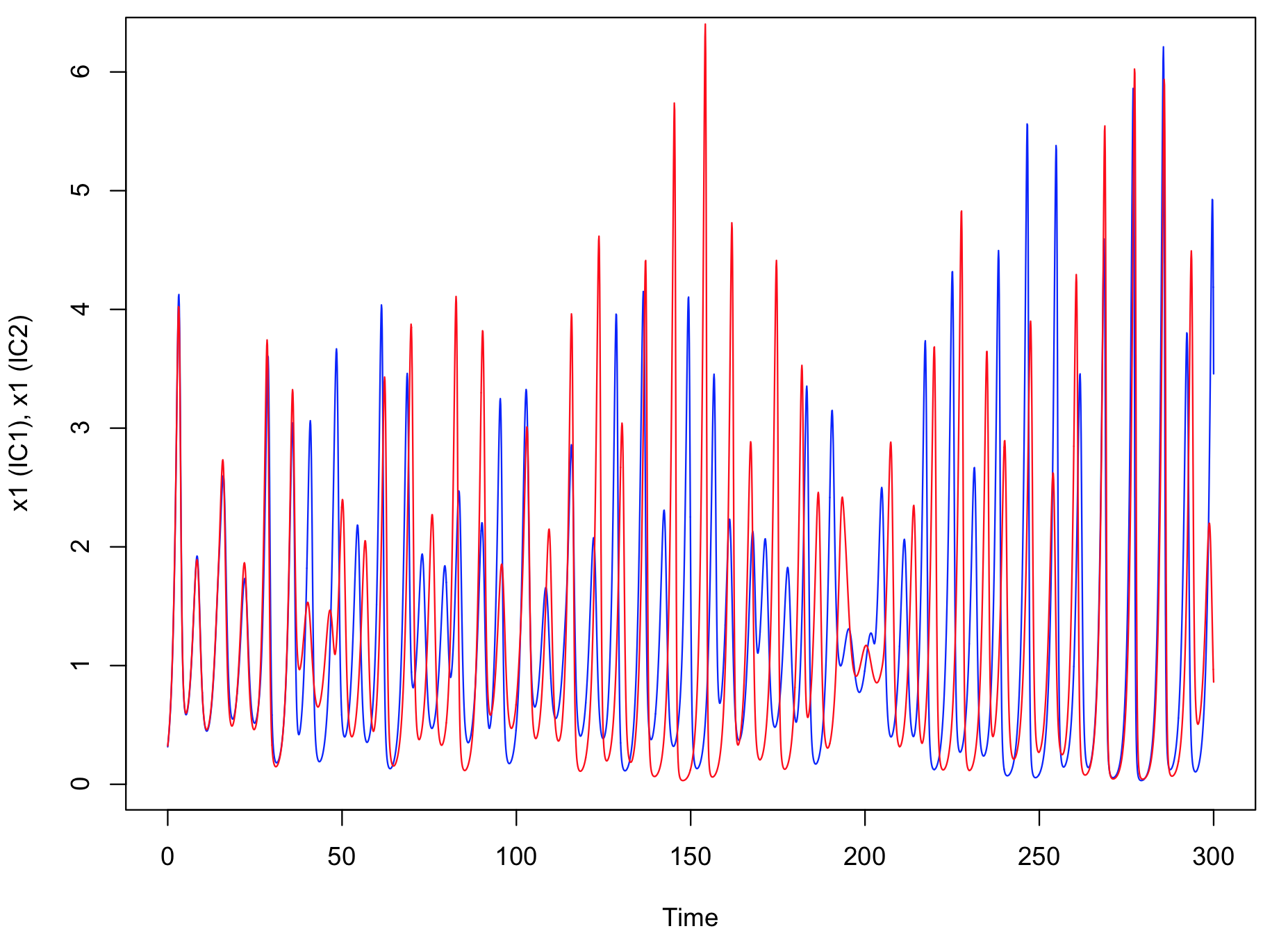
Sensitivity to initial conditions: Starting from different but close initial conditions, the trajectories progressively "diverge".
| R code |
b=c(1,-1,1,-1)


A=array(c(0,-1,0,0,1,0,0,-0.2,0,0,0,-1,0,0.2,1,0),c(4,4))

A=t(A)


ic1=runif(4)

ic2=ic1+0.01*runif(4)


R1=glv(N=4,A=A,b=b,tend=300,y=ic1)

R2=glv(N=4,A=A,b=b,tend=300,y=ic2)


time=as.numeric(colnames(R1))


plot(time,as.numeric(R1[1,]),col="blue",type="l",xlab="Time",ylab="x1 (IC1), x1 (IC2)")

lines(time,as.numeric(R2[1,]),col="red",type="l")
|
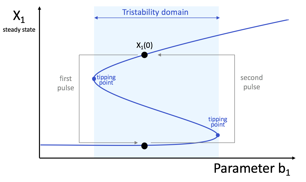
Multistability
The coexistence of multiple stables steady states (=multistability) can be illustrated with a variant of the Lotka-Volterra model in which the growth rates are described by "inhibitory" Hill function:
In this 3-species system, the growth of each species is inhibited by the two others. For the present practicals we will limit our analysis to this toy model but it can easily be generalized to N species.
Simulate this system for the following parameter values and for various initial conditions, and show the existence of tristability:
Kij = 0.1 ∀ i = j, n = 2, and ki = 0.1 ∀ i, b1 = 1, b2 = 0.95, b3 = 1.05.
Switches from one stable state to another can be induced by a transient change of a parameter value. Show that increasing b1 for a certain duration lead to a switch. What is the minimum value of b1 to observe the switch (tipping point)? How to induce the opposite switch? This illustrates the hysteresis effect.
Answer:
We first need to create an "ode" file with the modified equations:
| R code: glv2.R |
glv2<-function(t, N, parms){


K=0.1

kk=1

n=2

r=1

b1=1

b2=0.95

b3=1.05


f=c()


f[1]=K^n/(K^n+N[2]^n)*K^n/(K^n+N[3]^n)

f[2]=K^n/(K^n+N[1]^n)*K^n/(K^n+N[3]^n)

f[3]=K^n/(K^n+N[1]^n)*K^n/(K^n+N[2]^n)


dydt=c()


dydt[1] = r*N[1]*(b1*f[1]-kk*N[1])

dydt[2] = r*N[2]*(b2*f[2]-kk*N[2])

dydt[3] = r*N[3]*(b3*f[3]-kk*N[3])


list(dydt)


}  # end of function glv2
|
The following code can then be used to run a simulation for a given initial condition (y=...).
| R code |
tstart=0
tend=100
tstep=0.1
times<-seq(tstart, tend, by=tstep)
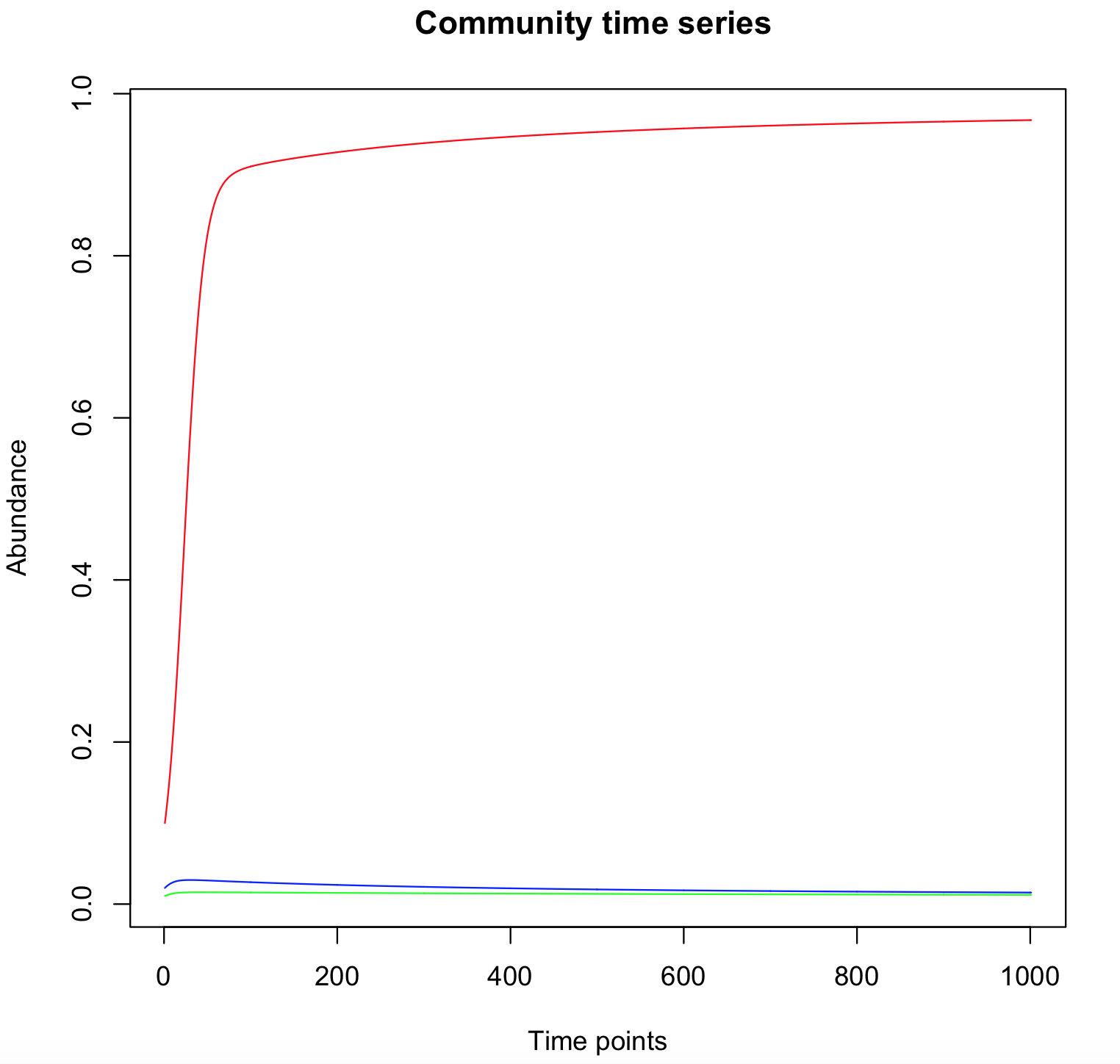
y=c(0.1,0.01,0.02) # initial condition (to be changed to illustrate tristabiliy)
parms=c()
R<-deSolve::lsoda(y, times, glv2, parms)
t=R[,1]
X=R[,2:ncol(R)]
X=t(X)
tsplot(X)
|
To highlight the tristability, run simulations with other initial condition and look at the "winning species".
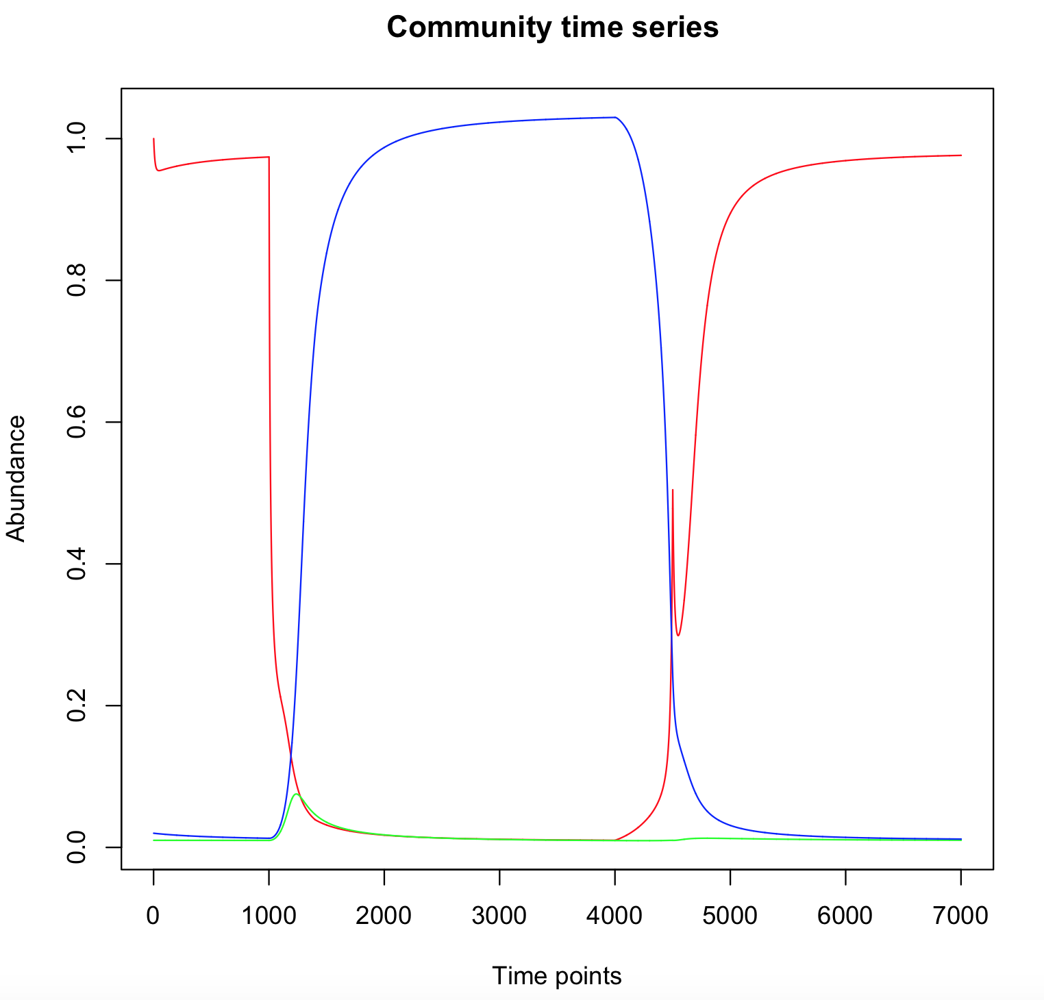
Here, two perturbations are directly implemented in the "ode" file. This is not a clean way to implement a perturbation, but it allows to rapidely check that transients perturbations can induce switches between steady states.
| R code: glv2perturb.R |
glv2perturb<-function(t, N, parms){


K=0.1

kk=1

n=2

r=1

b1=1

b2=0.95

b3=1.05


if ((t>100)&(t<140)) {

b1=0.2

}

else if ((t>400)&(t<450)){

b1=7.2

}


f=c()


f[1]=K^n/(K^n+N[2]^n)*K^n/(K^n+N[3]^n)

f[2]=K^n/(K^n+N[1]^n)*K^n/(K^n+N[3]^n)

f[3]=K^n/(K^n+N[1]^n)*K^n/(K^n+N[2]^n)


dydt=c()


dydt[1] = r*N[1]*(b1*f[1]-kk*N[1])

dydt[2] = r*N[2]*(b2*f[2]-kk*N[2])

dydt[3] = r*N[3]*(b3*f[3]-kk*N[3])


list(dydt)


} # end of funtion glv2perturb
|
| R code |
tstart=0

tend=700

tstep=0.1


times<-seq(tstart, tend, by=tstep)


y=c(1,0.01,0.02)   # initial condition (to be changed to illustrate tristabiliy)


parms=c()


R<-deSolve::lsoda(y, times, glv2perturb, parms)


t=R[,1]

X=R[,2:ncol(R)]

X=t(X)


tsplot(X)
|
References
- Benincŕ E, Ballantine B, Ellner SP, Huisman J (2015) Species fluctuations sustained by a cyclic succession at the edge of chaos. Proc Natl Acad Sci USA. 112:6389-94.
- Beninca E, Jöhnk KD, Heerkloss R, Huisman J. (2009) Coupled predator-prey oscillations in a chaotic food web. Ecol Lett. 12:1367-78.
- Coyte KZ, Schluter J, Foster KR (2015) The ecology of the microbiome: Networks, competition, and stability. Science 350:663-6.
- Gonze D, Lahti L, Raes J, Faust K. (2017) Multi-stability and the origin of microbial community types. ISME J. May 5.
- Solé RV and Bascompte J (2006) Self-Organization in Complex Ecosystems, Princeton Univ Press
- Vano JA, Wildenberg JC, Anderson MB, Noel JK, Sprott JC (2006) Chaos in low- dimensional Lotka-Volterra models of competition, Nonlinearity 19:2391-2404
Didier Gonze - 8/9/2017 - Summer School Leuven - September 2017
|